As machine learning (ML) systems become more integrated into our daily lives—from influencing who is hired to determining who qualifies for medical care—questions about fairness become impossible to ignore.
1.1 Why Fairness Matters?
ML systems learn from historical data, and history is not free of bias. If we are not careful, these models can magnify societal inequalities embedded in that data. Fairness in ML is about trying to prevent that. However, fairness is not a one-size-fits-all concept. Different fields define fairness in different ways:
Law: Fairness means protecting people from discrimination (e.g., based on race or gender).
Social sciences: Focus on systems of power and inequality—who gets advantages and who does not.
Computer science and statistics: Treat fairness as a math problem—something we can define and measure.
Philosophy and political theory: See fairness as a question of justice and moral reasoning.
1.2 Real-World Examples of Biased Algorithms
The COMPAS Algorithm Used in the US to predict which defendants are likely to reoffend, the COMPAS algorithm was designed to support bail and sentencing decisions. On the surface, it appeared fair—it was equally accurate for black and white defendants. However, an analysis by ProPublica revealed the following:
Black defendants who would not reoffend were twice as likely to be labeled “high risk.”
White defendants who did reoffend were often mislabeled “low risk.” Although the developers claimed that the model was fair (based on accuracy), it violated fairness in terms of racial bias, reinforcing systemic disparities.
Biased Healthcare Predictions In U.S. hospitals, an algorithm used to prioritize patients for preventative care relied on healthcare spending as a proxy for health needs. However, due to systemic disparities, black patients historically incurred lower medical costs—not due to better health, but due to under-treatment. As a result, the algorithm underestimated their needs, leading to biased care allocation.
2 How Do We Measure Fairness in ML?
Fairness in machine learning is typically categorized into two main types:
Group Fairness
Individual Fairness
2.1 Group Fairness
Group fairness ensures that different demographic groups (e.g., races or genders) are treated similarly by the model. A common metric used to quantify this is Demographic Parity, which aims for equal rates of positive outcomes across groups.
Demographic Parity Formula
Given two groups \(G_1\) and \(G_2\), and a binary classifier \(f : \mathbb{R}^p \to \{0, 1\}\), the deviation from demographic parity (DDP) is defined as:
A DDP of \(0\) indicates perfect demographic parity, meaning both groups receive positive outcomes at equal rates.
2.2 Individual Fairness
Individual fairness is based on the principle that similar individuals should receive similar outcomes. The main challenge lies in defining what it means for individuals to be “similar.” For example, should two loan applicants with identical incomes be considered similar if they differ in zip code or education level?
This definition is highly context-dependent and can be subjective, often requiring domain-specific knowledge to determine appropriate fairness constraints.
3 Raw Data and Fairness Metric for NBA Draft Selection Using ML
To evaluate fairness in NBA draft selections, we use college basketball data from 2009 to 2021.
Dataset Components
Player Performance Data: Points per game (PPG), assists (APG), shooting efficiency, etc.
Demographics: Height, school name, conference.
Draft Data: Draft round and pick number for selected players.
We merge the datasets by player name and year to construct a binary classification task: Was this player drafted (1) or not (0)?
3.1 Fairness Metric: Equal Opportunity for Drafting Talent
In a world where physical attributes and college brand often outweigh actual performance, we adopt Equal Opportunity as our fairness metric. In this context:
Players with comparable game statistics should have equal chances of being drafted, regardless of:
The prestige of their college (e.g., Davidson vs. Duke)
The conference in which they played (e.g., Southern vs. ACC)
Their physical traits, especially height (e.g., undersized guards often being overlooked)
3.2 Relevant Social Context: Biases in Scouting
The NBA draft process is deeply influenced by legacy scouting practices:
Size Bias: Overemphasis on height and athleticism can overlook highly skilled but smaller players.
Conference Prestige Bias: Players from smaller programs often receive less exposure and fewer opportunities.
Athletes like Steph Curry and Fred VanVleet exemplify players who may be unfairly penalized by traditional models. Our goal is to mitigate this through fairness-aware machine learning that recognizes talent irrespective of institutional pedigree.
3.3 Data Preprocessing and School Tier Annotation
We begin by merging two datasets: one containing college player statistics (2009–2021) and another listing NBA-drafted players during the same period. To ensure consistency, player names are standardized before matching. A binary ’Drafted‘ label is assigned based on presence in the official draft list.
To capture structural disparities across programs, we compute each school’s draft rate (number of players drafted divided by total players). Schools are then assigned to one of three tiers based on their draft rate quantiles:
Tier 1: Top 10% schools by draft rate
Tier 2: 60th to 90th percentile
Tier 3: Bottom 60%
This tier system enables group fairness evaluation across schools with varying institutional prestige.
Code
import pandas as pdimport reimport numpy as np# Load datacollege_df = pd.read_csv("CollegeBasketballPlayers2009-2021.csv")drafted_df = pd.read_excel("DraftedPlayers2009-2021.xlsx")# Standardize names for matchingcollege_df['player_name'] = college_df['player_name'].astype(str).str.strip().str.lower()drafted_df['PLAYER'] = drafted_df['PLAYER'].astype(str).str.strip().str.lower()# Add Drafted column: 1 if player in drafted list, 0 otherwisecollege_df['Drafted'] = college_df['player_name'].isin(drafted_df['PLAYER']).astype(int)def convert_excel_date_height(ht_str):# Convert month abbreviations to numbers month_map = {'jan': '01', 'feb': '02', 'mar': '03', 'apr': '04','may': '05', 'jun': '06', 'jul': '07', 'aug': '08','sep': '09', 'oct': '10', 'nov': '11', 'dec': '12' }try: ht_str =str(ht_str).lower()for month, number in month_map.items(): ht_str = ht_str.replace(month, number) parts = re.findall(r'\d+', ht_str)iflen(parts) ==2: inches, feet =map(int, parts)return feet *12+ inchesexcept:passreturn np.nan# Apply to create the height_in columncollege_df['height_in'] = college_df['ht'].apply(convert_excel_date_height)
The CVX optimization framework was employed to formulate and solve convex models underlying fairness-aware NBA draft prediction, including logistic regression variants (plain, ridge, lasso), support vector machines, and the FairStacks ensemble. By expressing these models as convex optimization problems, CVX enabled rapid prototyping without the need for custom algorithmic implementation.
Although Lasso regression is theoretically designed to drive some coefficients exactly to zero, solutions obtained via general-purpose solvers like CVX often yield near-zero coefficients due to numerical precision limitations. As a result, strict sparsity may require additional post-processing. Nevertheless, the framework provided sufficient flexibility to explore regularization effects and fairness constraints in the context of evaluating how players from less prestigious programs could be assessed more equitably based on game performance rather than institutional pedigree.
4.1 Implementation of the following classification methods as base learners to be used in construction of the FairStacks ensemble:
Naive Bayes (no CVX)
This implementation assumes conditional independence of features and fits Gaussian distributions separately for each class. The model computes:
Class-wise means (\(\mu_0\), \(\mu_1\)) and pooled variance \(\sigma^2\)
Prior class probabilities (\(\pi_0\), \(\pi_1\))
Log-likelihoods using the Gaussian log-density function
For each input vector, the model compares log-posterior probabilities and assigns a label of 1 if the class 1 posterior is greater, and 0 otherwise. This lightweight model is not only computationally simple but also provides useful diversity in the ensemble. Because Naive Bayes is so simple, it acts as a benchmark. If your complex models (like SVM or Lasso) don’t clearly outperform it, you might need to reassess their added complexity or feature use.
This implementation assumes Gaussian class-conditional distributions with a shared covariance matrix. LDA serves as a linear classifier that projects data to maximize class separability under these assumptions. The model performs the following:
Calculates class-wise means (\(\mu_0\), \(\mu_1\))
Computes the shared covariance matrix \(\Sigma\) across both classes
Solves the linear discriminant function (delta) for each class
Each data point is assigned to the class with the higher discriminant score. LDA offers a more flexible alternative to Naive Bayes by relaxing the independence assumption while still providing a computationally efficient, interpretable classifier.
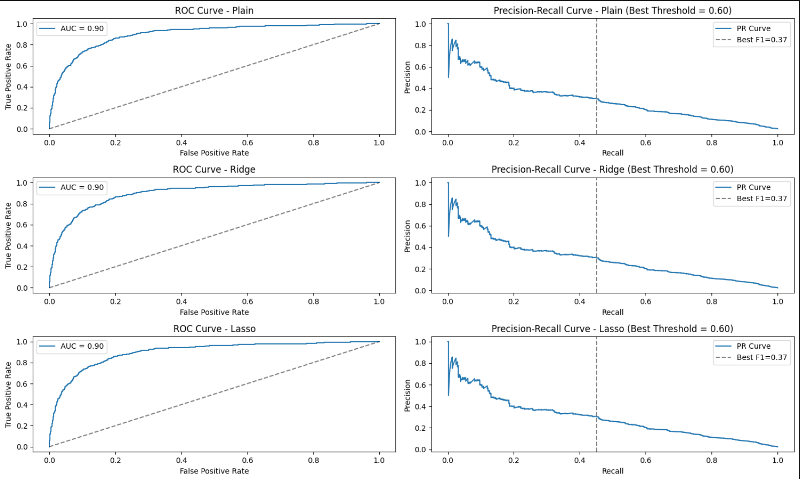
To model the probability of being drafted as a logistic function of player statistics, logistic regression was implemented using convex optimization. Three variants were considered: plain logistic regression, ridge-regularization, and lasso-regularization. The model minimizes the average logistic loss, with optional \(\ell_2\) or \(\ell_1\) penalty:
Plain: Minimizes standard logistic loss
Ridge: Adds \(\ell_2\) norm penalty to control weight magnitude
Lasso: Adds \(\ell_1\) norm penalty to encourage sparsity
Threshold tuning (e.g., using precision-recall curves) was applied to improve model calibration, especially when the dataset is imbalanced. A tuned threshold (e.g., 0.6) helps balance precision and recall based on evaluation metrics.
A regularization strength of \(\lambda = 0.1\) was selected as a reasonable value to balance overfitting and underfitting. It is strong enough to stabilize the solution but not so aggressive that it suppresses informative features.
ROC and Precision-Recall Curves for Plain, Ridge, and Lasso Logistic Regression (Best Threshold = 0.60)
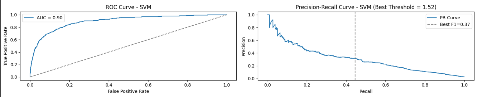
Support Vector Machine (SVM)
This implementation was developed using convex optimization with hinge loss and \(\ell_2\) regularization. This approach seeks to maximize the margin between classes while penalizing misclassifications near the decision boundary. The model performs the following:
Computes hinge loss \(\max(0, 1 - y_i x_i^\top \beta)\) for each point
Adds \(\ell_2\) regularization to prevent overfitting
Converts predictions from raw margin scores to 0/1 labels via thresholding
A decision threshold of 1.52 was selected empirically based on precision-recall and ROC curves to optimize performance. This allowed the classifier to maintain conservative positive predictions, especially useful in a fairness-aware pipeline where over-selection of dominant group members must be mitigated. A regularization parameter of \(\lambda = 0.1\) was chosen to softly penalize large weights while preserving flexibility in the decision boundary. This value was found to offer a stable trade-off between underfitting and overfitting in the fairness setting.
Code
def manual_svm_hinge(X_train, y_train, X_eval, lambda_=0.1):""" Train a linear SVM using hinge loss via CVXPY. - y_train should be in {0, 1} → converted internally to {-1, +1} - Returns 0/1 predictions for X_eval """ y_transformed =2* y_train -1# convert {0,1} to {-1,+1} n, p = X_train.shape beta = cp.Variable((p, 1)) margins = cp.multiply(y_transformed.reshape(-1, 1), X_train @ beta) hinge_loss = cp.sum(cp.pos(1- margins)) / n reg = lambda_ * cp.norm2(beta)**2 problem = cp.Problem(cp.Minimize(hinge_loss + reg)) problem.solve() raw_preds = X_eval @ beta.valuereturn (raw_preds >=1.52).astype(int).flatten()
ROC and Precision-Recall Curves for SVM (Best Threshold = 1.52)
Decision Tree
A decision tree classifier was included as a base learner using the built-in DecisionTreeClassifier from scikit-learn. This model makes hierarchical splits in the feature space to arrive at a decision path for each input. The implementation used the class_weight="balanced" argument to address class imbalance, ensuring the tree did not overly favor the majority class.
As we shift toward a fairness-aware ensemble strategy, it becomes critical to structure the data pipeline in a way that supports robust model selection and unbiased performance evaluation. Before learning ensemble weights or assessing bias mitigation, a principled strategy for dividing our dataset into training, validation, and test splits is essential.
This is especially important in the context of our Steph Curry fairness model, where the number of drafted players is relatively small and the fairness metric—True Positive Rate (TPR) gap between players from high-exposure programs (Tier 1) and lesser-known schools (Tier 3)—requires meaningful group-level comparisons. A careful partitioning ensures that the evaluation of how fairly we treat underdog players is accurate and unbiased.
To build a model that balances predictive power with fairness, we selected a combination of performance-based and context-aware features. Traditional box score statistics such as points per game, assists, steals, blocks, total rebounds, and shooting efficiency (eFG, TS per) were included to capture a player’s tangible on-court contributions. Additionally, height was included as a proxy for physical attributes that are often overvalued in the draft process.
Most importantly, we incorporated school tier—a categorical variable based on draft success rates of a player’s college program. This feature serves as the foundation for our fairness assessment, as we aim to detect and mitigate biases that favor players from elite programs (e.g., Duke, Kentucky) over similarly talented players from lesser-known schools (e.g., Davidson). Since our fairness metric is based on TPR disparities across school tiers, this feature is critical for evaluating whether players like Steph Curry, who came from a mid-major program, are systematically undervalued.
Base Learner Outputs and Stacking Matrix: Each of the seven base learners—Naive Bayes, Linear Discriminant Analysis (LDA), Decision Tree, three logistic regression variants (plain, ridge, lasso), and Support Vector Machine (SVM)—was trained on the training set and evaluated on the validation set. The binary predictions (0/1) of each learner on the validation set were vertically stacked to construct the matrix \(H_{\text{val}} \in \mathbb{R}^{n \times m}\), where \(n\) is the number of validation examples and \(m = 7\) is the number of base models. This matrix serves as input to the FairStacks optimization routine, allowing us to compute an ensemble prediction as a weighted combination of individual model decisions.
Fairness Vector Calculation: To estimate the bias of each base learner, we compute the True Positive Rate (TPR) separately for players from Tier 1 schools and those from lower-tier programs. The difference between these TPRs defines the bias for each learner:
Binary predictions from each model on the validation set are compared against ground truth labels, and group masks are applied to measure how fairly each learner treats players based on their school’s prestige. The resulting vector \(\hat{b}_j\) quantifies these group-level disparities and is used in the fairness penalty of the FairStacks objective.
Ensemble Weight Optimization via FairStacks:
With predictions and corresponding bias scores for each base learner in hand, the FairStacks optimization problem is solved to determine optimal ensemble weights. CVXPY is used to minimize a regularized logistic loss objective, where the penalty term is the absolute weighted sum of TPR gaps across base learners. The constraints ensure that all weights are non-negative and sum to one.
measures how well the ensemble predicts the true outcome \(y_i\) (drafted or not). Here, \(\hat{y}_i = \sum_j w_j \hat{f}_j(x_i)\) is the prediction from a weighted combination of base learners. The logistic loss is smooth and convex, making it ideal for binary classification tasks like draft prediction.
Fairness Penalty:
\[
\lambda \left| \sum_j w_j \hat{b}_j \right|
\]
penalizes disparity in treatment between groups—specifically, the absolute ensemble-weighted true positive rate (TPR) gap. Each \(\hat{b}_j\) represents the TPR gap of base learner \(j\), and minimizing this term encourages fairness across school tiers.
Constraints:
The weights \(\mathbf{w}\) form a convex combination \((w_j \geq 0, \sum_j w_j = 1)\), ensuring interpretability and stability.
Here, \(\lambda = 10\) emphasizes fairness by reducing group disparities between players from high-exposure and lower-tier programs. This balance is crucial in the Steph Curry fairness model, where the goal is to counteract systemic undervaluation of talented players from less visible schools.
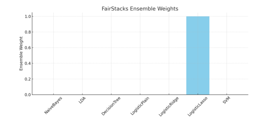
Final FairStacks Weights: [1.15064014e-10 1.02497679e-11 3.06854668e-13 5.65404680e-12
 6.72544450e-11 1.00000000e+00 8.35876761e-12]
Ensemble Test TPR Gap (Tier 1 vs Others): 0.0
0.9756941583587377
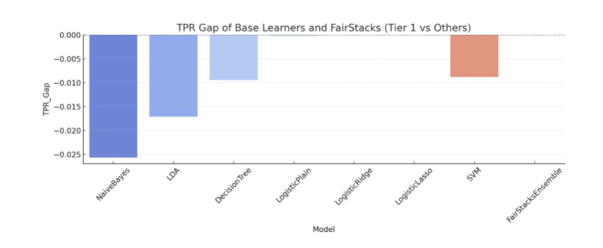
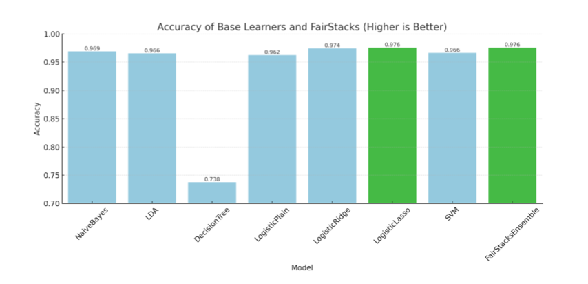
The final ensemble placed nearly all its weight on the Lasso-regularized logistic regression model. This outcome reflects the model’s ability to balance strong individual accuracy with fairness across school tiers. Despite the availability of other learners, including Decision Trees and SVMs, FairStacks effectively zeroed out their contributions to reduce potential TPR gaps. In terms of performance, the FairStacks ensemble matched the highest observed accuracy of 97.57% and achieved a TPR gap of 0.000. This is on par with Lasso regression alone, but with the added assurance that the model was selected through a fairness-aware optimization pipeline. Meanwhile, base learners such as Naive Bayes and LDA, despite respectable accuracy, exhibited substantial TPR gaps (e.g., -0.0256 and -0.0171), suggesting bias toward non-Tier 1 players. FairStacks thus succeeds in its dual objective: it preserves predictive performance while correcting for institutional bias, a key goal in fairness modeling for the NBA draft.
TPR Gap of Base Learners and FairStacks (Tier 1 vs Others)
Accuracy of Base Learners and FairStacks (Higher is Better)
---title: "STA 9890 Project: Ensemble Learning Techniques for Fair Classification"format: html: code-tools: true toc: true toc-depth: 3 code-fold: true math: true execute: echo: true output: true eval: false---# 1. Background on ML FairnessAs machine learning (ML) systems become more integrated into our daily lives—from influencing who is hired to determining who qualifies for medical care—questions about fairness become impossible to ignore.## 1.1 Why Fairness Matters?ML systems learn from historical data, and history is not free of bias. If we are not careful, these models can magnify societal inequalities embedded in that data. Fairness in ML is about trying to prevent that. However, fairness is not a one-size-fits-all concept. Different fields define fairness in different ways:- **Law**: Fairness means protecting people from discrimination (e.g., based on race or gender).- **Social sciences**: Focus on systems of power and inequality—who gets advantages and who does not.- **Computer science and statistics**: Treat fairness as a math problem—something we can define and measure.- **Philosophy and political theory**: See fairness as a question of justice and moral reasoning.## 1.2 Real-World Examples of Biased Algorithms**The COMPAS Algorithm** Used in the US to predict which defendants are likely to reoffend, the COMPAS algorithm was designed to support bail and sentencing decisions. On the surface, it appeared fair—it was equally accurate for black and white defendants. However, an analysis by ProPublica revealed the following:- Black defendants who would not reoffend were twice as likely to be labeled “high risk.” - White defendants who did reoffend were often mislabeled “low risk.”Although the developers claimed that the model was fair (based on accuracy), it violated fairness in terms of racial bias, reinforcing systemic disparities.**Biased Healthcare Predictions** In U.S. hospitals, an algorithm used to prioritize patients for preventative care relied on healthcare spending as a proxy for health needs. However, due to systemic disparities, black patients historically incurred lower medical costs—not due to better health, but due to under-treatment. As a result, the algorithm underestimated their needs, leading to biased care allocation.## 2 How Do We Measure Fairness in ML?Fairness in machine learning is typically categorized into two main types:- **Group Fairness**- **Individual Fairness**### 2.1 Group FairnessGroup fairness ensures that different demographic groups (e.g., races or genders) are treated similarly by the model. A common metric used to quantify this is **Demographic Parity**, which aims for equal rates of positive outcomes across groups.**Demographic Parity Formula** Given two groups $G_1$ and $G_2$, and a binary classifier $f : \mathbb{R}^p \to \{0, 1\}$, the deviation from demographic parity (DDP) is defined as:$$\text{DDP}(f) = \left| \mathbb{E}_{x \sim G_1}[f(x)] - \mathbb{E}_{x \sim G_2}[f(x)] \right|$$A DDP of $0$ indicates perfect demographic parity, meaning both groups receive positive outcomes at equal rates.### 2.2 Individual FairnessIndividual fairness is based on the principle that similar individuals should receive similar outcomes. The main challenge lies in defining what it means for individuals to be "similar." For example, should two loan applicants with identical incomes be considered similar if they differ in zip code or education level?This definition is highly context-dependent and can be subjective, often requiring domain-specific knowledge to determine appropriate fairness constraints.## 3 Raw Data and Fairness Metric for NBA Draft Selection Using MLTo evaluate fairness in NBA draft selections, we use college basketball data from 2009 to 2021.### Dataset Components- Player Performance Data: Points per game (PPG), assists (APG), shooting efficiency, etc.- Demographics: Height, school name, conference.- Draft Data: Draft round and pick number for selected players.We merge the datasets by player name and year to construct a binary classification task: **Was this player drafted (1) or not (0)?**### 3.1 Fairness Metric: Equal Opportunity for Drafting TalentIn a world where physical attributes and college brand often outweigh actual performance, we adopt Equal Opportunity as our fairness metric. In this context:Players with comparable game statistics should have equal chances of being drafted, regardless of:- The prestige of their college (e.g., Davidson vs. Duke)- The conference in which they played (e.g., Southern vs. ACC)- Their physical traits, especially height (e.g., undersized guards often being overlooked)### 3.2 Relevant Social Context: Biases in ScoutingThe NBA draft process is deeply influenced by legacy scouting practices:- Size Bias: Overemphasis on height and athleticism can overlook highly skilled but smaller players.- Conference Prestige Bias: Players from smaller programs often receive less exposure and fewer opportunities.Athletes like Steph Curry and Fred VanVleet exemplify players who may be unfairly penalized by traditional models. Our goal is to mitigate this through fairness-aware machine learning that recognizes talent irrespective of institutional pedigree.### 3.3 Data Preprocessing and School Tier AnnotationWe begin by merging two datasets: one containing college player statistics (2009–2021) and another listing NBA-drafted players during the same period. To ensure consistency, player names are standardized before matching. A binary ‘Drafted‘ label is assigned based on presence in the official draft list.To capture structural disparities across programs, we compute each school’s draft rate (number of players drafted divided by total players). Schools are then assigned to one of three tiers based on their draft rate quantiles:- Tier 1: Top 10% schools by draft rate - Tier 2: 60th to 90th percentile - Tier 3: Bottom 60%This tier system enables group fairness evaluation across schools with varying institutional prestige.```{python}import pandas as pdimport reimport numpy as np# Load datacollege_df = pd.read_csv("CollegeBasketballPlayers2009-2021.csv")drafted_df = pd.read_excel("DraftedPlayers2009-2021.xlsx")# Standardize names for matchingcollege_df['player_name'] = college_df['player_name'].astype(str).str.strip().str.lower()drafted_df['PLAYER'] = drafted_df['PLAYER'].astype(str).str.strip().str.lower()# Add Drafted column: 1 if player in drafted list, 0 otherwisecollege_df['Drafted'] = college_df['player_name'].isin(drafted_df['PLAYER']).astype(int)def convert_excel_date_height(ht_str):# Convert month abbreviations to numbers month_map = {'jan': '01', 'feb': '02', 'mar': '03', 'apr': '04','may': '05', 'jun': '06', 'jul': '07', 'aug': '08','sep': '09', 'oct': '10', 'nov': '11', 'dec': '12' }try: ht_str =str(ht_str).lower()for month, number in month_map.items(): ht_str = ht_str.replace(month, number) parts = re.findall(r'\d+', ht_str)iflen(parts) ==2: inches, feet =map(int, parts)return feet *12+ inchesexcept:passreturn np.nan# Apply to create the height_in columncollege_df['height_in'] = college_df['ht'].apply(convert_excel_date_height)``````{python}# --- TIER ASSIGNMENT BASED ON DRAFT RATE ---school_draft_stats = college_df.groupby('team')['Drafted'].agg(['sum', 'count'])school_draft_stats['draft_rate'] = school_draft_stats['sum'] / school_draft_stats['count']q90 = school_draft_stats['draft_rate'].quantile(0.90)q60 = school_draft_stats['draft_rate'].quantile(0.60)school_draft_stats['school_tier'] = pd.cut( school_draft_stats['draft_rate'], bins=[-1, q60, q90, 1.0], labels=['Tier 3', 'Tier 2', 'Tier 1'])college_df = college_df.merge(school_draft_stats['school_tier'], left_on='team', right_index=True, how='left')```## 4 Computation - CVX OptimizationThe CVX optimization framework was employed to formulate and solve convex models underlying fairness-aware NBA draft prediction, including logistic regression variants (plain, ridge, lasso), support vector machines, and the FairStacks ensemble. By expressing these models as convex optimization problems, CVX enabled rapid prototyping without the need for custom algorithmic implementation.Although Lasso regression is theoretically designed to drive some coefficients exactly to zero, solutions obtained via general-purpose solvers like CVX often yield near-zero coefficients due to numerical precision limitations. As a result, strict sparsity may require additional post-processing. Nevertheless, the framework provided sufficient flexibility to explore regularization effects and fairness constraints in the context of evaluating how players from less prestigious programs could be assessed more equitably based on game performance rather than institutional pedigree.### 4.1 Implementation of the following classification methods as base learners to be used in construction of the FairStacks ensemble:#### Naive Bayes (no CVX)This implementation assumes conditional independence of features and fits Gaussian distributions separately for each class. The model computes:- Class-wise means ($\mu_0$, $\mu_1$) and pooled variance $\sigma^2$- Prior class probabilities ($\pi_0$, $\pi_1$)- Log-likelihoods using the Gaussian log-density functionFor each input vector, the model compares log-posterior probabilities and assigns a label of 1 if the class 1 posterior is greater, and 0 otherwise. This lightweight model is not only computationally simple but also provides useful diversity in the ensemble. Because Naive Bayes is so simple, it acts as a benchmark. If your complex models (like SVM or Lasso) don’t clearly outperform it, you might need to reassess their added complexity or feature use.```{python}# --- MANUAL NAIVE BAYES ---def manual_gaussian_nb(X_train, y_train, X_test): X_0 = X_train[y_train==0] X_1 = X_train[y_train==1] mu_0, mu_1 = np.mean(X_0, axis=0), np.mean(X_1, axis=0) pi_0, pi_1 = X_0.shape[0] /len(X_train), X_1.shape[0] /len(X_train) pooled_var = (np.sum((X_0 - mu_0) **2, axis=0) + np.sum((X_1 - mu_1) **2, axis=0)) /len(X_train) pooled_var +=1e-6def log_gaussian(x, mu, var):return-0.5* np.sum(np.log(2* np.pi * var)) -0.5* np.sum(((x - mu) **2) / var)return np.array([1if np.log(pi_1) + log_gaussian(x, mu_1, pooled_var) > np.log(pi_0) + log_gaussian(x, mu_0, pooled_var) else0for x in X_test ])```#### Linear Discriminant Analysis (no CVX)This implementation assumes Gaussian class-conditional distributions with a shared covariance matrix. **LDA** serves as a linear classifier that projects data to maximize class separability under these assumptions. The model performs the following:- Calculates class-wise means ($\mu_0$, $\mu_1$)- Computes the shared covariance matrix $\Sigma$ across both classes- Solves the linear discriminant function (delta) for each classEach data point is assigned to the class with the higher discriminant score. LDA offers a more flexible alternative to Naive Bayes by relaxing the independence assumption while still providing a computationally efficient, interpretable classifier.```{python}# --- MANUAL LDA ---def manual_lda(X_train, y_train, X_test): X_0 = X_train[y_train ==0] X_1 = X_train[y_train ==1] mu_0, mu_1 = np.mean(X_0, axis=0), np.mean(X_1, axis=0) pi_0, pi_1 = X_0.shape[0] /len(X_train), X_1.shape[0] /len(X_train)# Regularized shared covariance matrix Sigma = ((X_0 - mu_0).T @ (X_0 - mu_0) + (X_1 - mu_1).T @ (X_1 - mu_1)) / (len(X_train) -2) Sigma +=1e-6* np.eye(Sigma.shape[0]) # small regularization to ensure invertibilitydef delta(x, mu, pi): a = np.linalg.solve(Sigma, mu)return x @ a -0.5* mu.T @ a + np.log(pi)return np.array([1if delta(x, mu_1, pi_1) > delta(x, mu_0, pi_0) else0for x in X_test ])```#### Logistic Regression (use CVX)To model the probability of being drafted as a logistic function of player statistics, logistic regression was implemented using convex optimization. Three variants were considered: plain logistic regression, ridge-regularization, and lasso-regularization. The model minimizes the average logistic loss, with optional $\ell_2$ or $\ell_1$ penalty:Plain: Minimizes standard logistic lossRidge: Adds $\ell_2$ norm penalty to control weight magnitudeLasso: Adds $\ell_1$ norm penalty to encourage sparsityThreshold tuning (e.g., using precision-recall curves) was applied to improve model calibration, especially when the dataset is imbalanced. A tuned threshold (e.g., 0.6) helps balance precision and recall based on evaluation metrics.A regularization strength of $\lambda = 0.1$ was selected as a reasonable value to balance overfitting and underfitting. It is strong enough to stabilize the solution but not so aggressive that it suppresses informative features.```{python}def logistic_cvx_preds_binary(X, y, X_eval, reg_type=None, lambda_=0.1, thresh=0.6): n, p = X.shape beta = cp.Variable((p, 1)) y_ = y.reshape(-1, 1) loss = cp.sum(cp.multiply(-y_, X @ beta) + cp.logistic(X @ beta))/nif reg_type =='ridge': penalty = lambda_ * cp.norm2(beta)**2elif reg_type =='lasso': penalty = lambda_ * cp.norm1(beta)else: penalty =0 cp.Problem(cp.Minimize(loss + penalty)).solve() probs =1/ (1+ np.exp(-X_eval @ beta.value))return (probs >= thresh).astype(int).flatten()```<div style="text-align: center;"> <img src="images/ROC Logistic Reg.png" alt="ROC Curves" width="100%"> <p><strong>ROC and Precision-Recall Curves for Plain, Ridge, and Lasso Logistic Regression</strong><br>(Best Threshold = 0.60)</p></div>#### Support Vector Machine (SVM)This implementation was developed using convex optimization with hinge loss and $\ell_2$ regularization. This approach seeks to maximize the margin between classes while penalizing misclassifications near the decision boundary. The model performs the following:- Computes hinge loss $\max(0, 1 - y_i x_i^\top \beta)$ for each point- Adds $\ell_2$ regularization to prevent overfitting- Converts predictions from raw margin scores to 0/1 labels via thresholdingA decision threshold of 1.52 was selected empirically based on precision-recall and ROC curves to optimize performance. This allowed the classifier to maintain conservative positive predictions, especially useful in a fairness-aware pipeline where over-selection of dominant group members must be mitigated. A regularization parameter of $\lambda = 0.1$ was chosen to softly penalize large weights while preserving flexibility in the decision boundary. This value was found to offer a stable trade-off between underfitting and overfitting in the fairness setting.```{python}def manual_svm_hinge(X_train, y_train, X_eval, lambda_=0.1):""" Train a linear SVM using hinge loss via CVXPY. - y_train should be in {0, 1} → converted internally to {-1, +1} - Returns 0/1 predictions for X_eval """ y_transformed =2* y_train -1# convert {0,1} to {-1,+1} n, p = X_train.shape beta = cp.Variable((p, 1)) margins = cp.multiply(y_transformed.reshape(-1, 1), X_train @ beta) hinge_loss = cp.sum(cp.pos(1- margins)) / n reg = lambda_ * cp.norm2(beta)**2 problem = cp.Problem(cp.Minimize(hinge_loss + reg)) problem.solve() raw_preds = X_eval @ beta.valuereturn (raw_preds >=1.52).astype(int).flatten()```<div style="text-align: center;"> <img src="images/ROC SVM.png" alt="ROC and PR Curves for SVM" width="100%"> <p><strong>ROC and Precision-Recall Curves for SVM</strong><br>(Best Threshold = 1.52)</p></div>#### Decision TreeA decision tree classifier was included as a base learner using the built-in `DecisionTreeClassifier` from scikit-learn. This model makes hierarchical splits in the feature space to arrive at a decision path for each input. The implementation used the `class_weight="balanced"` argument to address class imbalance, ensuring the tree did not overly favor the majority class.```{python}# --- DECISION TREE (BUILT-IN ALLOWED) ---tree_model = DecisionTreeClassifier(class_weight='balanced', random_state=0).fit(X_train, y_train)tree_preds = tree_model.predict(X_test)```## 5 Implementation and Assessment of FairstacksAs we shift toward a fairness-aware ensemble strategy, it becomes critical to structure the data pipeline in a way that supports robust model selection and unbiased performance evaluation. Before learning ensemble weights or assessing bias mitigation, a principled strategy for dividing our dataset into training, validation, and test splits is essential.This is especially important in the context of our Steph Curry fairness model, where the number of drafted players is relatively small and the fairness metric—True Positive Rate (TPR) gap between players from high-exposure programs (Tier 1) and lesser-known schools (Tier 3)—requires meaningful group-level comparisons. A careful partitioning ensures that the evaluation of how fairly we treat underdog players is accurate and unbiased.```{python}features = ['pts', 'ast', 'stl', 'blk', 'treb', 'height_in', 'TS_per', 'eFG', 'player_name', 'Drafted','school_tier']df = college_df[features].dropna()# --- SPLIT ---X = df.drop(columns=['Drafted', 'player_name'])y = df['Drafted']X_trainval, X_test, y_trainval, y_test = train_test_split(X, y, test_size=0.2, stratify=y, random_state=42)X_train, X_val, y_train, y_val = train_test_split(X_trainval, y_trainval, test_size=0.25, stratify=y_trainval, random_state=42)```To build a model that balances predictive power with fairness, we selected a combination of performance-based and context-aware features. Traditional box score statistics such as points per game, assists, steals, blocks, total rebounds, and shooting efficiency (eFG, TS per) were included to capture a player’s tangible on-court contributions. Additionally, height was included as a proxy for physical attributes that are often overvalued in the draft process.Most importantly, we incorporated school tier—a categorical variable based on draft success rates of a player’s college program. This feature serves as the foundation for our fairness assessment, as we aim to detect and mitigate biases that favor players from elite programs (e.g., Duke, Kentucky) over similarly talented players from lesser-known schools (e.g., Davidson). Since our fairness metric is based on TPR disparities across school tiers, this feature is critical for evaluating whether players like Steph Curry, who came from a mid-major program, are systematically undervalued.Base Learner Outputs and Stacking Matrix: Each of the seven base learners—Naive Bayes, Linear Discriminant Analysis (LDA), Decision Tree, three logistic regression variants (plain, ridge, lasso), and Support Vector Machine (SVM)—was trained on the training set and evaluated on the validation set. The binary predictions (0/1) of each learner on the validation set were vertically stacked to construct the matrix$H_{\text{val}} \in \mathbb{R}^{n \times m}$,where $n$ is the number of validation examples and $m = 7$ is the number of base models. This matrix serves as input to the FairStacks optimization routine, allowing us to compute an ensemble prediction as a weighted combination of individual model decisions.```{python}# Apply your functionsnb_val = manual_gaussian_nb_binary(X_train_raw, y_train.values, X_val_scaled)lda_val = manual_lda_binary(X_train_scaled, y_train.values, X_val_scaled)tree_val = DecisionTreeClassifier(max_depth=5, class_weight="balanced", random_state=0).fit(X_train_scaled, y_train).predict(X_val_scaled)log_plain_val = logistic_cvx_preds_binary(X_train_scaled, y_train.values, X_val_scaled)log_ridge_val = logistic_cvx_preds_binary(X_train_scaled, y_train.values, X_val_scaled, reg_type='ridge')log_lasso_val = logistic_cvx_preds_binary(X_train_scaled, y_train.values, X_val_scaled, reg_type='lasso')svm_val = manual_svm_hinge(X_train_scaled, y_train.values, X_val_scaled)# Build your H matrix using 0/1 predictionsH_val = np.vstack([nb_val, lda_val, tree_val, log_plain_val, log_ridge_val, log_lasso_val,svm_val]).T```Fairness Vector Calculation: To estimate the bias of each base learner, we compute the True Positive Rate (TPR) separately for players from Tier 1 schools and those from lower-tier programs. The difference between these TPRs defines the bias for each learner:```{python}# --- Fairness Vector ---tier_group = (X_val['school_tier'] =='Tier 1').astype(int)def compute_tpr_gap(y_true, y_scores, group, threshold=0.5): preds = (y_scores >= threshold).astype(int) mask_1 = group ==1 mask_0 = group ==0 tpr_1 = np.sum((preds[mask_1] ==1) & (y_true[mask_1] ==1)) / np.sum(y_true[mask_1] ==1) tpr_0 = np.sum((preds[mask_0] ==1) & (y_true[mask_0] ==1)) / np.sum(y_true[mask_0] ==1)return tpr_1 - tpr_0b_hat = np.array([ compute_tpr_gap(y_val.values, nb_val, tier_group), compute_tpr_gap(y_val.values, lda_val, tier_group), compute_tpr_gap(y_val.values, tree_val, tier_group), compute_tpr_gap(y_val.values, log_plain_val, tier_group), compute_tpr_gap(y_val.values, log_ridge_val, tier_group), compute_tpr_gap(y_val.values, log_lasso_val, tier_group), compute_tpr_gap(y_val.values, svm_val, tier_group)])```Binary predictions from each model on the validation set are compared against ground truth labels, and group masks are applied to measure how fairly each learner treats players based on their school’s prestige. The resulting vector $\hat{b}_j$ quantifies these group-level disparities and is used in the fairness penalty of the FairStacks objective.**Ensemble Weight Optimization via FairStacks:** With predictions and corresponding bias scores for each base learner in hand, the FairStacks optimization problem is solved to determine optimal ensemble weights. CVXPY is used to minimize a regularized logistic loss objective, where the penalty term is the absolute weighted sum of TPR gaps across base learners. The constraints ensure that all weights are non-negative and sum to one.$$\min_{\mathbf{w} \geq 0} \ \frac{1}{n} \sum_{i=1}^{n} \log \left( 1 + \exp(-y_i \cdot \hat{y}_i) \right) + \lambda \left| \sum_j w_j \hat{b}_j \right|, \quad \text{subject to} \quad \sum_j w_j = 1$$- **Logistic Loss Term:** $$ \frac{1}{n} \sum_{i=1}^{n} \log \left( 1 + \exp(-y_i \cdot \hat{y}_i) \right) $$ measures how well the ensemble predicts the true outcome $y_i$ (drafted or not). Here, $\hat{y}_i = \sum_j w_j \hat{f}_j(x_i)$ is the prediction from a weighted combination of base learners. The logistic loss is smooth and convex, making it ideal for binary classification tasks like draft prediction.- **Fairness Penalty:** $$ \lambda \left| \sum_j w_j \hat{b}_j \right| $$ penalizes disparity in treatment between groups—specifically, the absolute ensemble-weighted true positive rate (TPR) gap. Each $\hat{b}_j$ represents the TPR gap of base learner $j$, and minimizing this term encourages fairness across school tiers.- **Constraints:** The weights $\mathbf{w}$ form a convex combination$(w_j \geq 0, \sum_j w_j = 1)$, ensuring interpretability and stability. Here, $\lambda = 10$ emphasizes fairness by reducing group disparities between players from high-exposure and lower-tier programs. This balance is crucial in the Steph Curry fairness model, where the goal is to counteract systemic undervaluation of talented players from less visible schools.```{python}# --- FairStacks Optimization ---w = cp.Variable(H_val.shape[1])y_val_bin =2* y_val.values -1log_loss = cp.sum(cp.logistic(-cp.multiply(y_val_bin, H_val @ w))) /len(y_val)fairness_penalty = cp.abs(cp.sum(cp.multiply(w, b_hat)))lambda_ =10objective = cp.Minimize(log_loss + lambda_ * fairness_penalty)constraints = [w >=0, cp.sum(w) ==1]prob = cp.Problem(objective, constraints)prob.solve()final_weights = w.valueprint("Final FairStacks Weights:", final_weights)#--- Ensemble TPR Gap ---tier_group_test = (X_test['school_tier'] =='Tier 1').astype(int)ensemble_tpr_gap = compute_tpr_gap(y_test.values, ensemble_test_preds, tier_group_test)print("Ensemble Test TPR Gap (Tier 1 vs Others):", ensemble_tpr_gap)# --- Accuracy ---ensemble_accuracy = accuracy_score(y_test, ensemble_test_preds)print(ensemble_accuracy)``` Final FairStacks Weights: [1.15064014e-10 1.02497679e-11 3.06854668e-13 5.65404680e-12 6.72544450e-11 1.00000000e+00 8.35876761e-12] Ensemble Test TPR Gap (Tier 1 vs Others): 0.0 0.9756941583587377The final ensemble placed nearly all its weight on the Lasso-regularized logistic regression model. This outcome reflects the model’s ability to balance strong individual accuracy with fairness across school tiers. Despite the availability of other learners, including Decision Trees and SVMs, FairStacks effectively zeroed out their contributions to reduce potential TPR gaps.In terms of performance, the FairStacks ensemble matched the highest observed accuracy of 97.57% and achieved a TPR gap of 0.000. This is on par with Lasso regression alone, but with the added assurance that the model was selected through a fairness-aware optimization pipeline. Meanwhile, base learners such as Naive Bayes and LDA, despite respectable accuracy, exhibited substantial TPR gaps (e.g., -0.0256 and -0.0171), suggesting bias toward non-Tier 1 players. FairStacks thus succeeds in its dual objective: it preserves predictive performance while correcting for institutional bias, a key goal in fairness modeling for the NBA draft.<div style="text-align: center;"> <img src="images/TPR Gap Barplot.png" width="60%"> <p><strong>TPR Gap of Base Learners and FairStacks (Tier 1 vs Others)</strong></p></div><br><div style="text-align: center;"> <img src="images/Accuracy Barplot.png" width="60%"> <p><strong>Accuracy of Base Learners and FairStacks (Higher is Better)</strong></p></div><br><div style="text-align: center;"> <img src="images/Ensemble Weights Barplot.png" width="60%"> <p><strong>FairStacks Ensemble Weights</strong></p></div>## References1. Haas School of Business. *What is Fairness?*. University of California, Berkeley. Available at: [https://haas.berkeley.edu/wp-content/uploads/What-is-fairness_-EGAL2.pdf](https://haas.berkeley.edu/wp-content/uploads/What-is-fairness_-EGAL2.pdf) (Accessed April 2025).2. Michael Weylandt. *STA9890 Course Notes*. Available at: [https://michael-weylandt.com/STA9890/notes.html](https://michael-weylandt.com/STA9890/notes.html) (Accessed April 2025).3. Aditya K. *College Basketball Players 2009–2021*. Kaggle. Available at: [https://www.kaggle.com/datasets/adityak2003/college-basketball-players-20092021](https://www.kaggle.com/datasets/adityak2003/college-basketball-players-20092021) (Accessed April 2025).